Machine learning can guide food security efforts when primary data are not available

Target indicators

The two target indicators of the proposed predictive models—the prevalence of people with insufficient food consumption and the prevalence of people using crisis or above-crisis food-based coping—are calculated on the basis of two household-level indicators: the FCS³⁸ and the rCSI³⁹, respectively.

The FCS is calculated by asking each household how often, during the past seven days, it has consumed items from the different food groups: main staples, pulses, vegetables, fruit, meat and fish, milk, sugar, oil and condiments. Each consumption frequency is then weighted according to its relative nutritional importance to obtain the FCS = ∑w_ix_i, where w_i is the weight of food group i, and x_i is the frequency of its consumption by the household, that is, the number of days for which the food group was consumed during the past seven days. Once the food-consumption score is calculated, each household is then assigned a food-consumption group (poor, borderline or acceptable) based on standard thresholds, which can, however, be adapted based on specific consumption behaviours in the country of interest. Food group weights and thresholds are detailed in ref. ³⁸.

To compute the rCSI, households are asked if and how often during the past seven days they had to adopt the following coping behaviours: relying on less-preferred or less-expensive food, borrowing food from relatives or friends, limiting portion sizes, restricting adults’ consumption for small children to eat and reducing the number of meals eaten in a day. Coping strategy frequencies are then weighted according to their severity to obtain the rCSI, as detailed in ref. ³⁹.

The available historical data for the two indicators have statistical representativeness at the spatial resolution of first-level administrative units and have been collected through both face-to-face and mobile phone surveys, including those from WFP’s near-real time monitoring systems. Because the mode of questionnaire administration can have serious effects on data quality⁴⁰, post-stratification weighting schemes are applied by WFP to surveys collected in a remote fashion to mitigate sampling and modality bias, as detailed in ref. ⁴¹. The prevalence of people with insufficient food consumption and the prevalence of people using crisis or above-crisis food-based coping are then obtained as the weighted prevalence of households in the sample with, respectively, poor or borderline food consumption and with rCSI ≥ 19 (ref. ⁴²).

The insufficient food-consumption data span units across 78 countries from 2006 to July 2021, and the crisis or above food-based coping data units across 41 countries from 2013 to July 2021, with more than 200,000 observations for each indicator. This large volume of data is, however, not equally representative of all covered geographical areas: countries where a WFP’s near-real time monitoring system is in place are over-represented because these systems provide data on a daily basis, whereas in the remaining countries, data collection is performed only a few times per year. Therefore, to avoid training the models on an unbalanced dataset, sampling is performed by randomly selecting, for each first-level administrative unit, five observations per month only. The final dataset used to train and test the models where the prevalence from previous assessments is not included as an independent variable is composed of 37,926 observations for food consumption and 35,894 for food-based coping. For the models where the prevalence from a previous assessment is instead included, the size is further reduced because only observations preceded by a previous one can be used, resulting in 24,510 observations for food consumption and 12,570 for food-based coping. The breakdown by country of all of the above-mentioned numbers is reported in Supplementary Table 1.

Feature definition and selection

The initial set of considered features is composed of variables related to food insecurity and its main drivers: economic shocks, extreme weather events and conflict¹¹. Because the goal of the models is to provide interpretable insights to decision-makers, the guiding principle for feature definition was expert opinion. To include as much variety as possible in terms of potential drivers, a manual, expert-guided, minimal feature selection process was performed, as detailed below. Let us note that such an approach is not expected to remove all multi-collinearity, but a tree-based method (XGboost) that is robust to multi-collinearity⁴³ was subsequently used.

Food prices

To capture variations in cereal and tuber prices, we resort to the Alert for Price Spikes (ALPS) indicator⁴⁴. This metric is based on a trend analysis of monthly price data: the idea is to compare the long-term seasonal trend of a commodity’s price time series in a market with the last observed price in the same market, providing an indication of the intensity of the difference between the current market price and the historical trend. The higher the difference, the more severe the alert. Price data and the corresponding ALPS calculations are publicly available through WFP’s Economic Explorer platform⁴⁵. If more than one market is present within a geographical area, the average ALPS value is considered. If no market is instead monitored in a given area, the national average is considered. From these data, we build a set of three features by taking into account the minimum, maximum and average ALPS value within a three-month window. The length of the window was selected as the shortest time period that minimizes the number of missing values in the training and test set. A one-month lag is applied to ensure data availability when deploying the model in real time. Because the three defined features are different variants of the same indicator, and they display high levels of positive correlation (Spearman’s correlation coefficients ρ > 0.85 for all three combinations), only one was selected as independent variable for the models. The selected variable is the maximum ALPS value, being the one with the highest correlation with the target indicators (correlations were computed using the training data only).

Macro-economic indicators

The following four macro-economic features are considered: most-recent available annual GDP per capita in a four-year time window, most-recent available monthly headline and food inflation rates in a six-month time window (applying a one-month lag) and percentage variation between the average value of the currency exchange rate during the past three months and the average value during the previous three, to capture main changes in the situation. The three-month window was selected for consistency with the food price features, and the same applies to the following features too. Being all country-level indicators, the same national value is assigned to all first-level administrative units within a country. Data are obtained from Trading Economics, a website providing publicly available economic and financial indicators, including historical data, for 196 countries⁴⁶. For countries where unofficial currency exchange rate is collected by WFP, these values are used instead of official ones⁴⁷, because they provide a more reliable representation of the country’s economic situation.

Weather

An initial set of five weather features is built by taking: (1) the average rainfall and normalized difference vegetation index (NDVI) during a 12-month time window, which allows characterization of each first-level administrative unit’s climate; (2) rainfall and NDVI anomalies with respect to historical averages. For rainfall, two anomalies have been defined by WFP: the ratio between the amount of rainfall during the past one month or three months and the historical average of the amount of rainfall in the same period of the year. For NDVI, a single anomaly is defined based on the past ten days, because vegetation already integrates the effects of previous rainfall. All three anomalies are provided for each ten-day window of the year, and we take their average during a three-month window as for previous features, applying a ten-day lag. Data are obtained from WFP’s Seasonal Explorer platform⁴⁸, which provides open rainfall and NDVI time series for a near-global set of administrative units, computed, respectively, from the Climate Hazards Group InfraRed Precipitation with Station data (CHIRPS)⁴⁹ and the Moderate Resolution Imaging Spectroradiometer (MODIS)⁵⁰ data. In this case, similar to food prices, the defined features are different variants of the same two indicators, and a correlation analysis was performed to reduce their number. Between the two averages during a 12-month time window (ρ = 0.93), the average NDVI was selected as the most correlated with the target indicators. Similarly, between the two rainfall anomalies (ρ = 0.82), the one-month anomaly was selected. Finally, the NDVI anomaly was also selected given its low correlation with the other four variables (ρ < 0.4 in all cases).

Conflict

Conflict data are obtained from the Armed Conflict Location and Event Data Project, a publicly available repository of reported conflict events and related fatalities across most areas of the world⁵¹. The date, latitude and longitude of each event is reported, allowing it to match to the corresponding first-level administrative unit. To capture deterioration or improvements in the conflict situation, we define the conflict features as the difference between the number of reported fatalities during the past three months and the three months prior, applying a 14-day lag. Only fatalities reported in events involving organized violence (that is ‘battles’, ‘violence against civilians’ and ‘explosions/remote violence’) are considered⁵², and a total of seven features is obtained by considering these three categories separately and in combination. Again, a correlation analysis was performed in the same fashion as for the previous cases, and only the ‘violence against civilians’ feature was selected as an independent variable for the models.

Prevalence of under-nourishment

The most-recent available prevalence of under-nourishment in a four-year time window is considered. This is a national yearly indicator publicly available in the Food and Agriculture Organization Corporate Statistical Database (FAOSTAT)⁵³. Being a country-level indicator, the same national value is assigned to all first-level administrative units within a country.

Population density

Yearly population density is also considered and obtained from the Center for International Earth Science Information Network (CIESIN) raster files⁵⁴ by averaging all pixel values within each first-level administrative unit. Estimates for years not covered by the dataset are obtained through linear interpolation.

Previous value of the target indicator

Finally, the previously measured prevalence of people with insufficient food consumption and of people using crisis or above-crisis food-based coping are also considered, when available. For first-level administrative units where WFP’s near-real time monitoring is in place, only data collected before the start of the near-real time monitoring is used to build this feature. This choice was made because the proposed models are meant to be used in practice in situations where no near-real time monitoring is in place, and hence the last-available value would be from a face-to-face or mobile phone assessment conducted in a specific and limited time window in the past.

Modelling approach

The proposed models predict the probability of having a person with insufficient food consumption or using crisis or above-crisis food-based coping in a given area at a given time. The objective function is therefore a logistic curve. Gradient Boosted Decision Trees⁵⁵ was identified as the most suitable algorithm to perform the regressions, given its high performance, flexibility and its capacity to handle complex and nonlinear relationships. The XGboost implementation was used²⁵.

Four different models were developed: two for the prevalence of people with insufficient food consumption and two for the prevalence of people using crisis or above-crisis food-based coping. In each case, one includes the prevalence from a previous assessment as independent variable, and one does not.

That is, in the first model, the dependent variable is the prevalence of people with insufficient food consumption in a given first-level administrative area a at a given date d, and the corresponding independent variables are: (1) the last-available prevalence of people with insufficient food consumption in area a at a time before d (and before the start of the near-real time monitoring, if this is in place in area a); (2) the most-recent prevalence of under-nourishment (in a four-year time window) available at date d for the country that area a is part of; (3) the most-recent annual GDP per capita (in a four-year time window) available at date d for the country that area a is part of; (4) the most-recent headline inflation rate (in a six-month time window) available at date d for the country that area a is part of; (5) the most-recent food inflation rate (in a six-month time window) available at date d for the country that area a is part of; (6) the percentage variation between the average value of the currency exchange rate during the three months preceding date d and the average value during the previous three for the country that area a is part of; (7) the maximum ALPS value in area a for the three months before date d; (8) the average NDVI in area a during the 12 months before date d; (9) the average one-month rainfall anomaly in area a for the three months before date d; (10) the average NDVI anomaly in area a for the three months before date d; (11) the difference between the number of reported fatalities in violence against civilians events in area a during the three months preceding date d (minus a 14-day lag) and the three months prior; (12) the most-recent population density estimate for area a available at date d. The second model has the same dependent variable and all the same independent variables except the first one (that is, the last-available prevalence of insufficient food consumption). In the third model, the prevalence of people using crisis or above-crisis food-based coping in a given first-level administrative area a at a given date d is the dependent variable, and the independent variables are the same as above, except the first variable, which is instead the last-available prevalence of people using crisis or above-crisis food-based coping in area a at a time before d (and before the start of the near-real time monitoring, if this is in place in area a). Finally, in the fourth model, the dependent variable is the same as in the third, and the independent variables are all the variables (2) to (12).

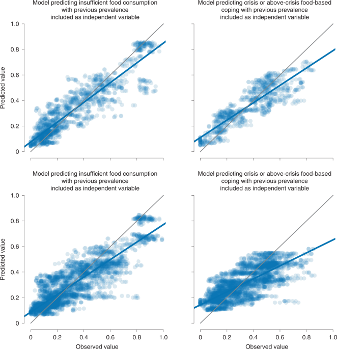
For each model, the following procedure was performed. The data were split into two parts following their temporal ordering: data until 31 May 2021 (corresponding to ~85% of the data) were used for training and validation, and the remaining two months (~15% of the data) for testing. To tune the model hyper parameters, a walk-forward validation approach was used: four folds were created, each covering one month of data, from February through May 2021, and for each fold, the training set was composed of all the older data up to the end of the previous month. The tuned hyper parameters and the explored values are listed in Supplementary Table 2. The chosen combination of hyper parameters is the one leading to the smallest difference between the average R² on the folds used as training set and the average R² on the folds used as validation. We opted for this criterion to favour models where the performance on the test is the most similar to the performance on the training set because large differences are often an indication of overfitting. Once the hyper parameters are selected, N_b = 100 models are fitted on samples with replacement of the training and validation set (that is, bootstrapping), and the test set is used to evaluate the model’s performance. For each observation in the test set, N_b predictions are generated (one per bootstrapped model), and the median value is then used to calculate the model performance metrics, that is, the coefficient of determination R² and the mean absolute error (MAE), which are reported in Table 1 and Fig. 1. Supplementary Figs. 152–155 show that convergence for both metrics is reached within 100 bootstraps.

SHAP values

SHAP (SHapley Additive exPlanations)²⁸ is a framework recently proposed to interpret predictions made by often complex black box machine learning algorithms. SHAP unifies other methods (Lime, DeepLift and so on), and for tree-based models, it allows for writing a prediction as the sum of a baseline value and each feature’s contribution²⁹:

SHAP values for tree-based models such as XGboost have been shown to improve on other local tree explanations, such as visualizing the decision tree, which is not feasible for tree ensembles, and on model-agnostic local explanations, which are computationally expensive if explaining large datasets²⁹. Moreover, SHAP local explanations can be used as building blocks for global explanations, as shown in Supplementary Fig. 1, where we take the mean absolute value of SHAP values across all data points to build a global feature-importance ranking. In this study, we use the Python open-source implementation of the TreeSHAP algorithm⁵⁶.

Explaining the single prediction

SHAP values represent each feature’s contribution towards the model prediction, and their absolute value can therefore be interpreted as each feature’s importance. This method improves on widely used global feature-importance methods such as split-based or gain-based measures, as it allows computation of prediction-specific feature importance. As detailed in previous sections, each of our four models actually consists of N_b = 100 different models fitted on different samples (with replacement) of the training data, of which we report the median prediction and confidence interval. To determine the importance of a feature, we then take each feature’s median SHAP value across the N_b bootstrapped models. Convergence checks are reported in Supplementary Figs. 156–157.

In this study, predictions are originally obtained at the spatial resolution of first-level administrative units, but they can then be aggregated to display results at the national level, too. To determine feature importance at the country level, we average the SHAP values across all first-level administrative units in a country by weighting each value according to the unit’s population. This can be easily interpreted: a SHAP value corresponds to the change in prevalence with respect to the baseline due to one feature. By performing a population-based weighted average, we are computing the change in number of people due to that feature. This operation then sums the number of people across all units and divides it by the country population to return the change in national prevalence. The same operation is also performed on the model baseline. Note that this also allows us to combine predictions coming from areas with and without a previous value of the target variable, even if the underlying models use slightly different sets of features.

Explaining trend changes

This method allows us to compute the feature-importance ranking for a given area in a given day, explaining which features were the most important and how they contributed to the final prediction. However, predictions for the same area can produce a trend in time, which, in turn, can show changes in prevalence due to changes in the input variables. We extend the SHAP framework to explain which features are responsible in determining changes in predicted trends.

Let us take two predictions y^t1 and y^t2 corresponding to the same area but two different dates. Following equation (1), we can write the trend change y^t2 − y^t1 in terms of the change χ_i in SHAP values relative to each of the M features:

The features with largest associated SHAP value change are the ones that determined the trend change. Moreover, the sign of the change χ_i also tells us whether that feature has caused an increase or decrease in the prevalence, that is, a deterioration or improvement in the food security situation.

Note that equation (2) is exact when considering a single model for a single first-level administrative area but is only an approximation when considering median SHAP values, as previously mentioned. It is also important to note that this method can give apparently misleading indications due to nonlinear interactions between features. For instance, a feature that does not change value between the two dates can be the one with the largest SHAP value change (that is, determining the trend change). This happens because other features change value, thus changing its relative importance in the two predictions. One could overcome this limitation by computing SHAP interaction values²⁹, but the computation is not feasible when dealing with our sample size, that is, 400 models (100 bootstrapped iterations per model) and daily computations. Moreover, this would imply dealing with an order of 50 (number of features squared, divided by 2) different interactions, which would greatly undermine our effort to produce explainable predictions for decision-makers.

Reporting summary

Further information on research design is available in the Nature Research Reporting Summary linked to this article.